Stock Price Analysis and Visualization in Python
Python is a high-level, interpreted programming language known for its readability, simplicity, and versatility. Created by Guido van Rossum and first released in 1991, Python has become one of the most popular programming languages in the world. Its design philosophy emphasizes code readability with its notable use of significant whitespace.
Python’s simplicity, readability, and versatility, combined with strong community support and a wide range of applications, make it an ideal programming language for beginners.
Preparation
An Integrated Development Environment (IDE) is a software application that provides comprehensive facilities to computer programmers for software development. An IDE typically consists of a source code editor, build automation tools, and a debugger. Some IDEs also offer intelligent code completion, linting (for identifying potential errors), and version control integration.
- PyCharm: PyCharm is an integrated development environment used for programming in Python. It provides code analysis, a graphical debugger, an integrated unit tester, integration with version control systems, and supports web development with Django.
- Jupyter Notebook: The Jupyter Notebook is the original web application for creating and sharing computational documents. It offers a simple, streamlined, document-centric experience.
- Google Colab: Colab is a hosted Jupyter Notebook service that requires no setup to use and provides free access to computing resources, including GPUs and TPUs.
- Visual Studio Code: A versatile and lightweight code editor that supports Python and many other languages. It’s highly customizable and has a vast extension library.
- Spyder: Popular within the scientific community, integrates well with scientific packages like NumPy, SciPy, and Matplotlib.
- Anaconda: Not an IDE itself, but a distribution of Python and R for scientific computing. It simplifies package management and deployment and includes Jupyter and Spyder.
When choosing an IDE for Python development, the best choice depends on your specific needs, preferences, and the nature of your project. If you are a professional developer working on large-scale applications, PyCharm might be the best choice. For data science, machine learning, and scientific computing where interactive data exploration and visualization are key, Jupyter Notebook or Google Colab are excellent choices. If you want a balance between a traditional IDE and a tool for data science, Visual Studio Code or Spyder might be the right fit.
Typically, you should install Python before installing an Integrated Development Environment (IDE) for Python development. Usually, you download and install Python from python.org. During installation, ensure you select the option to add Python to your system path. After Python is installed, you can choose and install an IDE of your preference. The IDE will use the Python interpreter installed on your system.
If you are installing PyCharm, it can detect existing Python installations or even download and set up Python if you do not have it already. If you are using the Anaconda distribution, it comes with Python and a suite of other useful data science packages. Anaconda also includes Spyder and Jupyter Notebook, so you won’t need to install Python separately.
Google Colab runs in the cloud and provides a Python environment that is ready to use — you do not need to install Python on your machine.
Meanwhile, Visual Studio Code (VS Code) requires Python to be installed on your system. VS Code will detect the Python interpreter installed on your machine. If you are planning to use Jupyter Notebook through Anaconda, separate Python installation is not necessary as Anaconda already includes Python. If you want to use Jupyter independently, you will need Python installed first.
How to Approach Stock Price Analysis and Visualization in Python
Stock price analysis and visualization in Python is an exciting and highly relevant application of programming in the field of finance. Python, with its powerful libraries like Pandas, Matplotlib, and Seaborn, provides an accessible platform for performing these tasks.
To analyze stock prices, the first step is to obtain historical stock data. You can use APIs like Yahoo Finance, Alpha Vantage, or Quandl to fetch this data. Python libraries like yfinance (specifically for Yahoo Finance) make it easy to download this data directly into Python. You can also manually download and fetch the data from Yahoo Finance.
Import Libraries
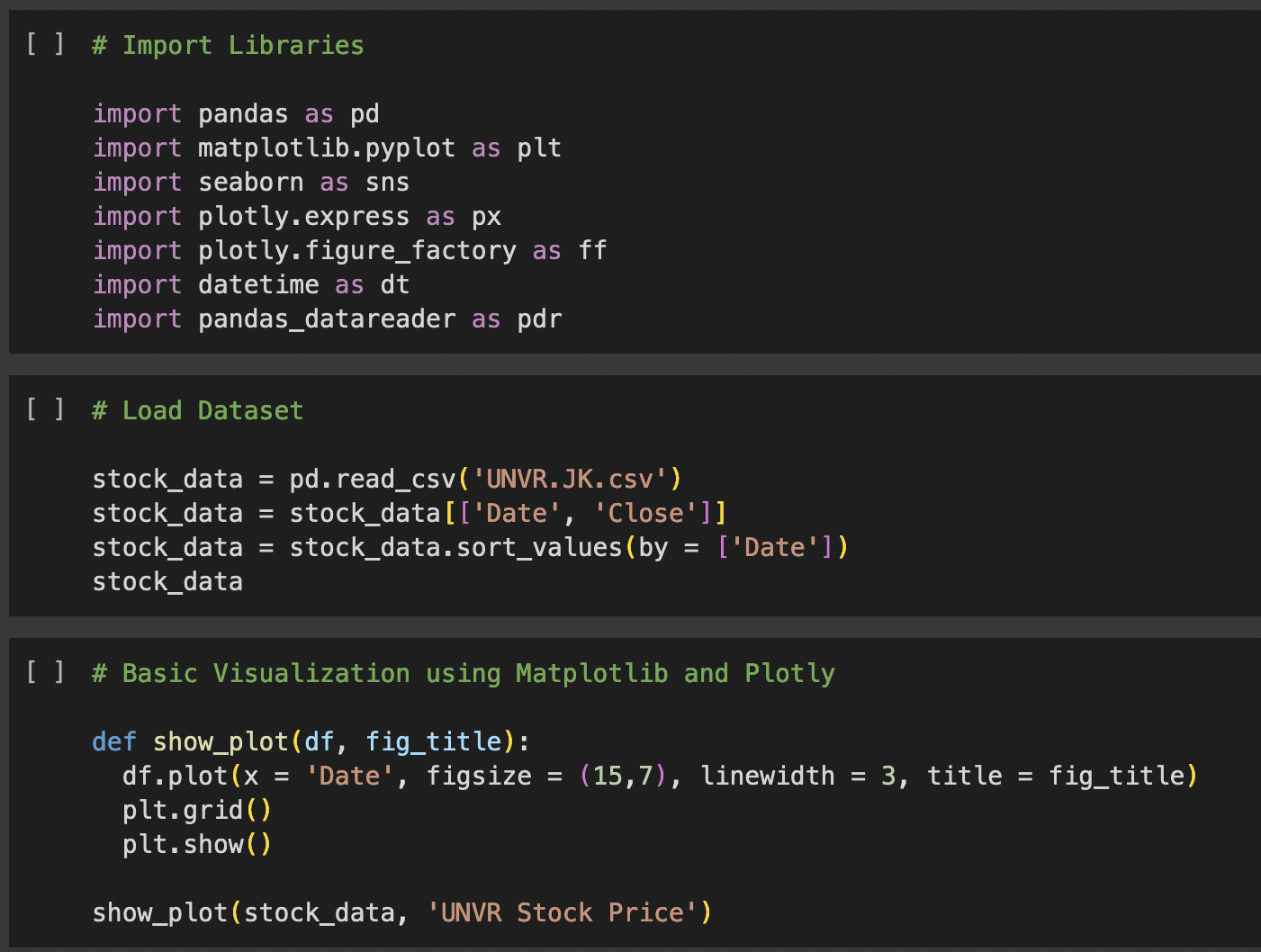
This section imports various Python libraries needed for the script:
- pandas for data manipulation.
- matplotlib.pyplot and seaborn for data visualization.
- plotly.express and plotly.figure_factory for interactive plots.
- datetime for handling date and time data.
- pandas_datareader for fetching financial data from various sources.
# Import Libraries
import pandas as pd
import matplotlib.pyplot as plt
import seaborn as sns
import plotly.express as px
import plotly.figure_factory as ff
import datetime as dt
import pandas_datareader as pdr
Load Dataset
This part loads a CSV file containing stock data (specifically for the ticker UNVR.JK) into a pandas DataFrame. It then selects only the ‘Date’ and ‘Close’ columns and sorts the data based on the ‘Date’ column.
# Load Dataset
stock_data = pd.read_csv(‘UNVR.JK.csv’)
stock_data = stock_data[[‘Date’, ‘Close’]]
stock_data = stock_data.sort_values(by = [‘Date’])
stock_data
Basic Visualization using Matplotlib and Plotly
This function show_plot creates a basic line plot of the stock prices using Matplotlib. It sets the figure size, line width, and title, and then displays the plot.
# Basic Visualization using Matplotlib and Plotly
def show_plot(df, fig_title):
df.plot(x = ‘Date’, figsize = (15,7), linewidth = 3, title = fig_title)
plt.grid()
plt.show()
show_plot(stock_data, ‘UNVR Stock Price’)
Interactive Plot using Matplotlib and Plotly
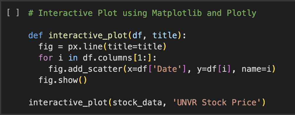
The interactive_plot function creates an interactive line plot using Plotly. It iterates through each column in the DataFrame (except ‘Date’) and adds them as separate scatter plots to the figure.
# Interactive Plot using Matplotlib and Plotly
def interactive_plot(df, title):
fig = px.line(title=title)
for i in df.columns[1:]:
fig.add_scatter(x=df[‘Date’], y=df[i], name=i)
fig.show()
interactive_plot(stock_data, ‘UNVR Stock Price’)
Load Dataset More
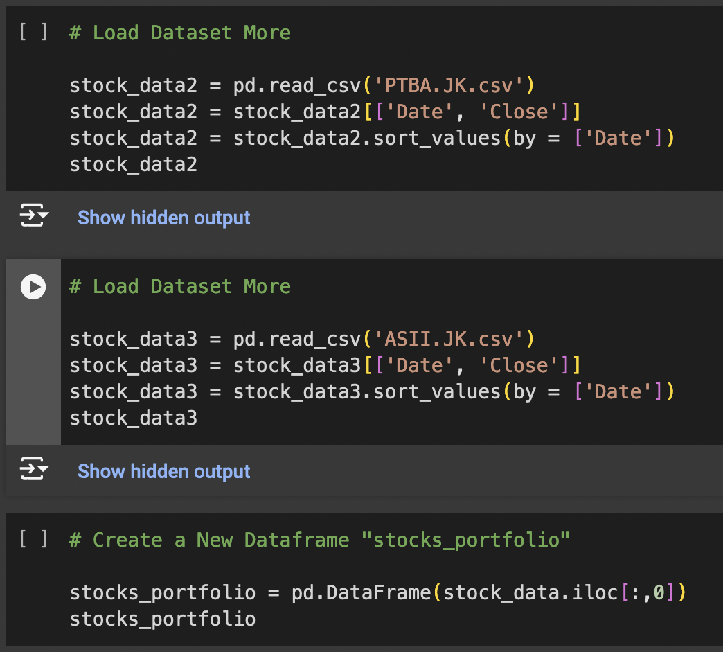
These sections load additional datasets for other stock tickers (PTBA.JK and ASII.JK) and process them in the same way as the first dataset.
# Load Dataset More
stock_data2 = pd.read_csv(‘PTBA.JK.csv’)
stock_data2 = stock_data2[[‘Date’, ‘Close’]]
stock_data2 = stock_data2.sort_values(by = [‘Date’])
stock_data2
# Load Dataset More Again
stock_data3 = pd.read_csv(‘ASII.JK.csv’)
stock_data3 = stock_data3[[‘Date’, ‘Close’]]
stock_data3 = stock_data3.sort_values(by = [‘Date’])
stock_data3
Create a New Dataframe “stocks_portfolio”
This creates a new DataFrame stocks_portfolio containing only the ‘Date’ column from stock_data.
# Create a New Dataframe “stocks_portfolio”
stocks_portfolio = pd.DataFrame(stock_data.iloc[:,0])
stocks_portfolio
Append Close Price from Each Stock to the “stocks_portfolio”
This part adds the ‘Close’ price columns for each stock ticker to the stocks_portfolio DataFrame.
# Append Close Price from Each Stock to the “stocks_portfolio”
stocks_portfolio[‘UNVR’] = stock_data.iloc[:,1]
stocks_portfolio[‘PTBA’] = stock_data2.iloc[:,1]
stocks_portfolio[‘ASII’] = stock_data3.iloc[:,1]
stocks_portfolio

Normalize Stock Portfolio and Visualize It
The normalize function normalizes the stock prices relative to their initial values. It then uses the interactive_plot function to visualize the normalized data.
# Normalize Stock Portfolio and Visualize It
def normalize(df):
x = df.copy()
for i in x.columns[1:]:
x[i] = x[i]/x[i][0]
return x
interactive_plot(normalize(stocks_portfolio), ‘Stocks Portfolio’)

Calculate Overall Portfolio Return
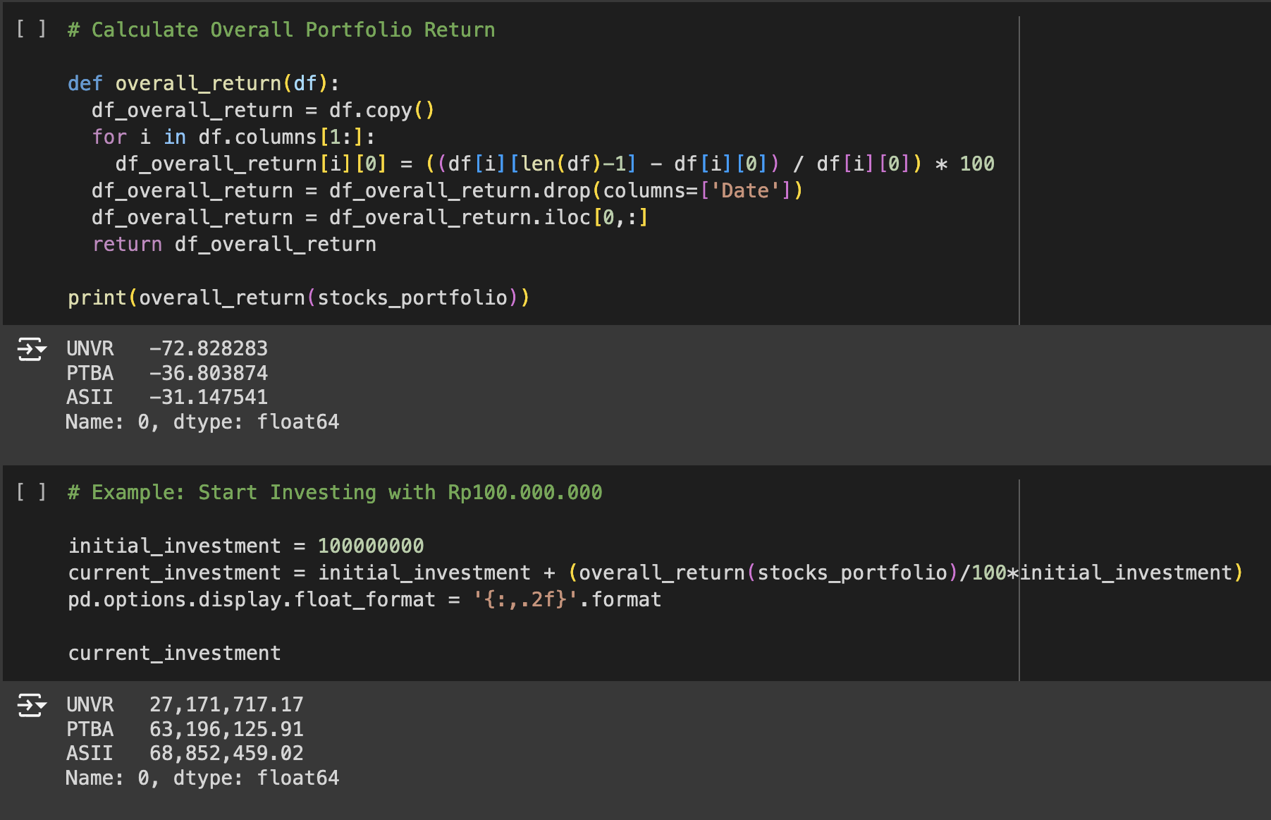
This function calculates the overall return of each stock in the portfolio as a percentage.
# Calculate Overall Portfolio Return
def overall_return(df):
df_overall_return = df.copy()
for i in df.columns[1:]:
df_overall_return[i][0] = ((df[i][len(df)-1] – df[i][0]) / df[i][0]) * 100
df_overall_return = df_overall_return.drop(columns=[‘Date’])
df_overall_return = df_overall_return.iloc[0,:]
return df_overall_return
print(overall_return(stocks_portfolio))
Example: Start Investing with Rp100.000.000
This section calculates the current value of an initial investment based on the overall returns of the stock portfolio.
# Example: Start Investing with Rp100.000.000
initial_investment = 100000000
current_investment = initial_investment + (overall_return(stocks_portfolio)/100*initial_investment)
pd.options.display.float_format = ‘{:,.2f}’.format
current_investment
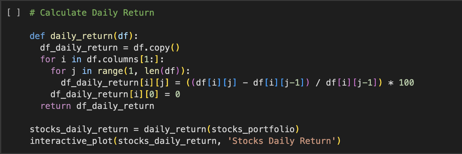
Calculate Daily Return
The daily_return function calculates the daily returns of each stock in the portfolio. It then visualizes these daily returns using the interactive_plot function.
# Calculate Daily Return
def daily_return(df):
df_daily_return = df.copy()
for i in df.columns[1:]:
for j in range(1, len(df)):
df_daily_return[i][j] = ((df[i][j] – df[i][j-1]) / df[i][j-1]) * 100
df_daily_return[i][0] = 0
return df_daily_return
stocks_daily_return = daily_return(stocks_portfolio)
interactive_plot(stocks_daily_return, ‘Stocks Daily Return’)
Heatmap Analysis
This code creates a heatmap of the correlation matrix for the daily returns of the stocks in the portfolio using Seaborn.
# Heatmap Analysis
cm = stocks_daily_return.drop(columns=[‘Date’]).corr()
plt.figure(figsize=(10,10))
sns.heatmap(cm, annot=True)

Visualize Daily Return
This line generates histograms for the daily returns of each stock in the portfolio.
# Visualize Daily Return
stocks_daily_return.hist(figsize=(10,10), bins=40);

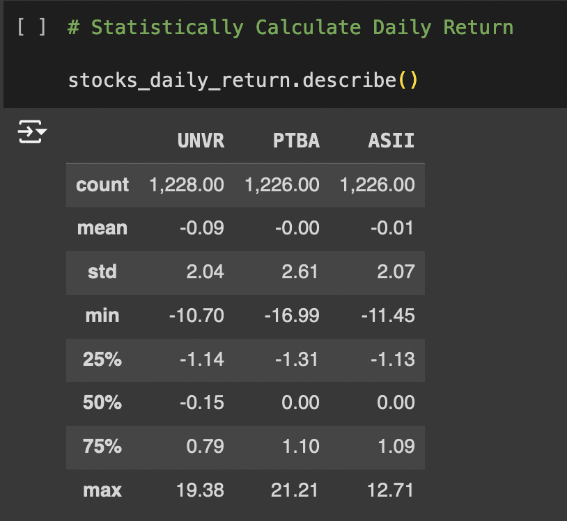
Statistically Calculate Daily Return
Finally, describe() is used to display descriptive statistics for the daily returns of the stocks.
# Statistically Calculate Daily Return
stocks_daily_return.describe()
Overall, this script provides a (rather) comprehensive approach to analyzing and visualizing stock data in Python, from basic data processing to more advanced analyses and visualizations.
Stock price analysis in Python is a blend of data analysis and financial knowledge. It requires not only the ability to write Python code and use libraries but also a fundamental understanding of the stock market and financial concepts. Remember, while Python can provide powerful tools for analysis, it is essential to complement these tools with sound financial judgment and risk management.
Support and Resources
To support the learning of Python, Pandas, and data visualization, I recommend a combination of online courses, tutorials, and YouTube videos. These resources are designed to cater to beginners and provide a solid foundation in these areas.
- Python.org’s Beginner’s Guide: A great starting point for complete beginners, offering various resources and documentation.
- Corey Schafer’s Python Tutorial for Beginners: A comprehensive Python tutorial series that covers basics in a clear, easy-to-understand manner.
- Sentdex’s Data Analysis with Python and Pandas: A tutorial series covering various aspects of data visualization using Python.
- Data School’s Data Analysis in Python with Pandas: A series of videos covering the essentials of Pandas for data manipulation.
- DataCamp’s Introduction to Pandas: A hands-on course to learn Pandas for data analysis.
- Matplotlib Official Tutorials: Official tutorials for learning Matplotlib, a fundamental library for data visualization in Python.
- Seaborn Official Documentation: Seaborn is built on top of Matplotlib and provides a high-level interface for drawing attractive and informative statistical graphics.
These resources will help you grasp the fundamentals and apply them in practical scenarios. Remember, the key to learning programming is consistent practice and application of concepts in real-world problems.